Instrumentation

img-harvard_forest-instrumentation.jpg

img-harvard_forest-instrumentation-1.jpg
The automated Environmental Monitoring Station (EMS) monitors the concentration of a variety of chemical species, in addition to general environmental measurements. These species include NOy, NOx, CO2, H2O, O3, CO, and several different hydrocarbons (For a complete list see the table below). We measure the net flux hourly aggregating to seasons, years, and decades. Methods used to calculate concentrations include infrared and UV-Vis spectrophotometry, chemiluminescence, and gas chromatography.  Measurements of carbon dioxide and trace gases have been nearly continuous since 1990, and data through 1999 is publicly available through our data exchange.

Schematic representation of the CO2 eddy measurement.

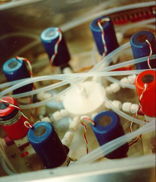
This schematic representation of the CO2 eddy measurement shows how the CO2 measurement is calibrated by standard addition. A small flow of calibration gas is added to the sample flow of 5-6 lpm. The pressure in the detector cell is measured and controlled. Total flow in the system is measured in order to identify periods with filter clogging and to do the calibration calculations. Calibration of NOx and NOy measurements also use standard addition and have similar plumbing.

 8 inlets are arranged from 30 cm to 30m on or near the tower.
8 inlets are arranged from 30 cm to 30m on or near the tower. Each inlet is selected in turn by activating a solenoid on the "hub" pictured above. Teflon is used to minimize alteration of O3 and NOx concentrations. The entire sampling line is at a constant reduced pressure to prevent condensation of water vapor.

For more information about our instruments and how we make our measurements contact Bill Munger or John Budney.

List of sensors and quantities measures on eddy-flux tower at Harvard Forest.

Sensor inlet/ instrument altitudes determined quantity (data rate) Dates Active
ATI Sonic Anemometer
30m
Three-dimensional wind velocity, temperature, momentum & heat fluxes (30-min avg)
Ongoing
NOy (catalyst-->NO)
30m
NOy fluxes, 30-minute averages 
1992-2002
high-speed CO2-H2O IR-Absorbance
30m
CO2 and H2O fluxes (30-min avg)
Ongoing
high-speed O3 C2H4 - chemiluminescence
30m
Ozone flux (30-min avg)
1992-2002
slow CO2 IR absorbance
30,24,18,12,6,
3,1,0.05m
CO2 concentration along a vertical profile
(8 levels @ 2/hr)
Ongoing
slow O3 UV absorbance
30,24,18,12,6,
3,1,0.05 m
O3 concentration along a vertical profile
(8 levels @ 2/hr)
Ongoing
slow NOx (Photolysis, O3-chemiluminescence)
30,24,18,12,6,
3,1,0.05m
NO, NO2 concentration along a vertical profile (8 levels @ 2/hr)
1992-2002 and intermittently since
Thermistor, thin-film capacitor
30,22,12,6,
3m
Temperature and relative humidity profile (5,60-min avg)
Ongoing
Thermistors
surface (6 reps),
20cm, 50cm
soil temperatures (5,60-min avg) 
Ongoing
PAR sensors
30,12m
photosynthetically active radiation
(5,60-min avg) 
Ongoing
Net radiometer
30m
net radiative heat flux (5,60-min avg) 
Ongoing
CO Gas-filter correlation IR absorbance
30m
CO concentrations (4,60-min avg) 

Dasibi 1992-2002

Teledyne 2012-present

GC-FID
30m
1CH4 concentrations(60-min avg)
1992-1994 Shipham et al 1998
2-Channel GC-FID
29,24m 
gradient for fluxes
C2-C6 hydrocarbon concentrations (2/hr)
4-Channel GC-ECD (FACTS)
29m
Halocarbons, N2O, CO, CH4, SF6
1-channel GC
30m
 PAN
suspended
Tuneable Diode laser absorption spectrometer
30m
NO2 and HNO3
2000
Quantum Cascade Laser absorption spectrometer
30m
NO2 and HONO
2011
/* Harvard Forest breadcrumb */ #block-boxes-1628108821 a, #block-boxes-1628108821 a:visited { color: #ffffff; margin-left: 6.05em; background-color: #4d5d71; padding: .5em 1em .3em 1em; } /* Grid layout of "list of posts" widget */ .node { margin-bottom: 20px; display: inline-grid; } /* Hide "Read more" links */ #columns a.node-readmore { border-bottom: none; font-weight: bold; padding-right: 11px; position: relative; z-index: 9; text-decoration: none; font-size: .90em; display: none; } /* Hide "..." next to images */ #columns p:only-child { margin: 0 0px .4em; color: #fff; } /* Center align links above images */ .block-boxes-os_sv_list_box h1.node-title { margin-bottom: 0; text-align: center; } /* No image padding-right */ img.media-element.file-default { padding-right: 0px; margin: 0 1em; } /* Larger links to sub pages */ .block-boxes-os_sv_list_box h1.node-title { margin-bottom: .5em; text-align: center; font-size: x-large; margin-left: 1em; margin-right: 1em; } /* Hide link to taxonomy */ .field-name-og-vocabulary { display: none; } /* "The Site" layout of images */ .media-element-container { height: auto !important; margin: 0 1em 0 1em; display: inline-block; } /* "The Site" center align image figcaption */ img ~ figcaption { color: #555; font-style: italic; clear: both; max-width: 100%; text-align: center; padding-left: 1em; } /* "The Site" h2 */ h2 { line-height: 1.2em; margin: 2em 0 -1.5em 0; } /* Accordion links */ h3.ui-accordion-header { font-family: 'Droid Sans', sans-serif !important; font-size: x-large; color: #215990; } /* Slideshow descriptions */ #layout_16_9_side .slide { background: #4444441f; border: medium none; border-radius: 0 0 0 0; box-shadow: 0 0 0 0 rgb(0 0 0 / 85%); position: relative; z-index: 2; } #layout_16_9_side .slide-copy { background: #000000 !important; clear: none; float: right; padding-top: 4%; position: relative; width: 38.5%; z-index: 4; /* color: #000000 !important; */ } /* Footer */ /* Footer */ .three-3x33 > .region { width: 27%; }